Technical Projects
Strategic Bidding in a Congested Power System: A Bayesian Game Approach
Project: Game-Theoretic Analysis of Generator Bidding Behavior in Wholesale Electricity Markets, Tokyo Eastern Cement Company (Pvt) Ltd, Trincomalee
Tools: Renewable Energy Integration, Power System Analysis, Optimal Power Flow (OPF), Probabilistic Modeling, Game Theory, Python
This project models the strategic bidding behavior in a wholesale electricity market where a conventional Independent Power Producer (IPP) and a Renewable Energy (Wind) generator compete. The core challenge addressed is asymmetric information: the Wind generator has private knowledge of its exact available generation capacity, whereas the IPP must bid blindly, relying solely on prior probabilistic beliefs about the wind states.
1. Model Parameters & Optimal Power Flow (OPF) Data
The fundamental parameters of the game establish the physical generation limits, the cost structure, and the probabilities of the hidden states of nature.
-
Maximum Capacities:
- Grid Generator (Bus 1 - Slack Bus): 9999 MW. This acts as an effectively infinite capacity connection to ensure the grid can always balance load deficits and transmission losses.
- IPP Generator (Bus 2 - Gas): 100 MW. This is the absolute physical capacity of the plant, which is fully offered when the IPP chooses the "Aggressive" bidding action.
- Wind Generator (Bus 3 - Renewable): 60 MW. This represents the maximum generation achievable when Nature dictates a "High" wind state (which drops to 10 MW during a "Low" wind state).
- Marginal Costs: IPP = $30.0/MWh, Wind = $0.0/MWh.
- Probabilities of Nature's States: High Wind = 0.6, Low Wind = 0.4.
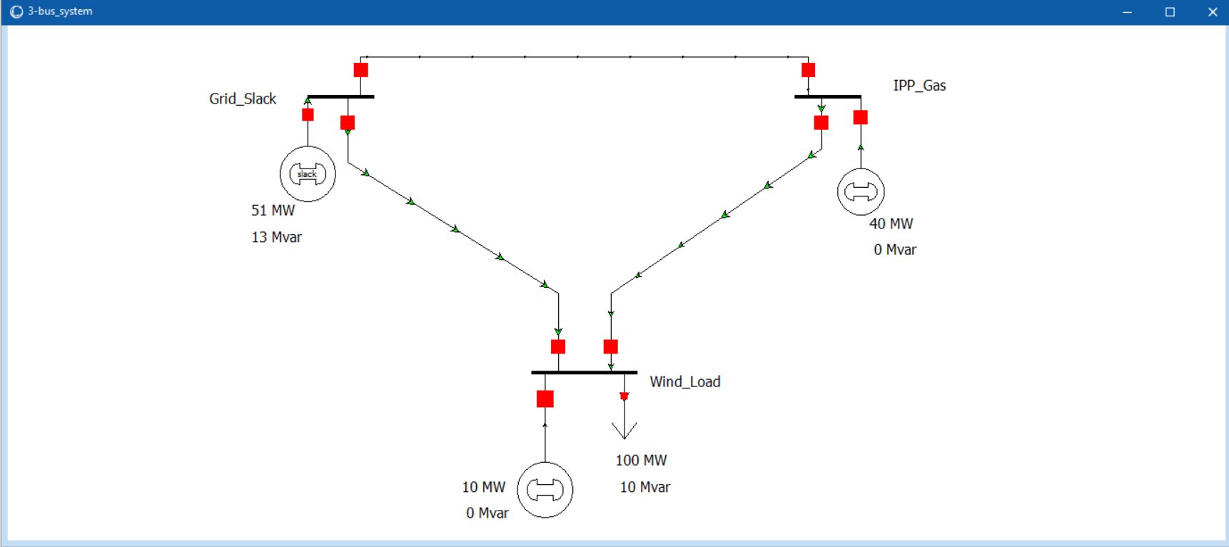
The payoffs are derived from a simulated physical Optimal Power Flow (OPF) using PowerWorld Simulator24 software. Below is the raw structural OPF dataset representing [LMP IPP, Dispatch IPP, LMP Wind, Dispatch Wind] under all possible action profiles and states:
| Wind State | IPP Action | Wind Action | LMP IPP ($/MWh) | Disp IPP (MW) | LMP Wind ($/MWh) | Disp Wind (MW) |
|---|---|---|---|---|---|---|
| High Wind (60 MW) | Conservative (40 MW) | Withhold (0 MW) | 80.0 | 40.0 | 80.0 | 0.0 |
| Max (60 MW) | 80.0 | 40.0 | 80.0 | 60.0 | ||
| Aggressive (100 MW) | Withhold (0 MW) | 80.0 | 100.0 | 80.0 | 0.0 | |
| Max (60 MW) | 41.0 | 40.0 | 41.0 | 60.0 | ||
| Low Wind (10 MW) | Conservative (40 MW) | Withhold (0 MW) | 80.0 | 40.0 | 80.0 | 0.0 |
| Max (10 MW) | 80.0 | 40.0 | 80.0 | 10.0 | ||
| Aggressive (100 MW) | Withhold (0 MW) | 80.0 | 100.0 | 80.0 | 0.0 | |
| Max (10 MW) | 91.0 | 91.0 | 41.8 | 10.0 |
2. Perfect Information Payoffs
The utility function for each player is defined as their net operational profit:
Ui(aIPP, aWind, θ) = (LMPi × Dispatchi) - (Marginal Costi × Dispatchi)
Applying this formula to the OPF data yields the exact Ex-Post payoffs (UIPP, UWind) assuming perfect information of the wind state:
State: High Wind (θHigh = 0.6)
| IPP \ Wind | Withhold | Max |
|---|---|---|
| Conservative | (2000, 0) | (2000, 4800) |
| Aggressive | (5000, 0) | (440, 2460) |
State: Low Wind (θLow = 0.4)
| IPP \ Wind | Withhold | Max |
|---|---|---|
| Conservative | (2000, 0) | (2000, 800) |
| Aggressive | (5000, 0) | (5551, 418) |
Therefore, the strategy mapping to play Max under all conditions, denoted as MM (Max, Max), is strictly dominant.
3. Expected Utility (Bayesian Normal Form)
Because the IPP acts without knowing the true wind state, we evaluate its decisions against the four composite strategies available to the Wind player (e.g., "WM" denotes Withholding in High wind, but bidding Max in Low wind). The Ex-Ante Expected Utility (EU) represents a probability-weighted average:
E[U] = 0.6 × UHigh + 0.4 × ULow
| IPP \ Wind Strategy | WW (Withhold, Withhold) |
WM (Withhold, Max) |
MW (Max, Withhold) |
MM (Max, Max) |
|---|---|---|---|---|
| Conservative | (2000, 0) | (2000, 320) | (2000, 2880) | (2000, 3200) |
| Aggressive | (5000, 0) | (5220.4, 167.2) | (2264, 1476) | (2484.4, 1643.2) |
- EUIPP(Conservative | MM) = 2000.0
- EUIPP(Aggressive | MM) = 2484.4
4. Algorithm: Compute Pure-Strategy Bayesian Nash Equilibrium
To programmatically determine the market equilibrium, the theoretical framework is implemented using the following computational steps to evaluate all possible strategy spaces:
Output: Equilibrium Profile (s*IPP, s*Wind)
// Phase 1: Compute Payoffs Conisdering Perfect Information
FOR EACH state θ ∈ {High, Low}:
// Phase 2: Construct Expected Utility Matrix
DEFINE WindStrategies sWind ∈ {WW, WM, MW, MM}
FOR EACH sIPP ∈ {Conservative, Aggressive}:
// Phase 3: Identify Mutual Best Responses (BNE)
FOR EACH player i ∈ {IPP, Wind}:
RETURN matching profiles (s*IPP, s*Wind)
5. Equilibrium Analysis: Get the Upper Bound of the Threshold Probability (p*)
Proposition
Let p ∈ [0, 1] represent the probability of the High Wind state (θHigh) and 1 - p represent the probability of the Low Wind state (θLow). The strategic bidding game yields a unique pure-strategy Bayesian Nash Equilibrium (BNE) that is strictly dependent on the threshold probability p* ≈ 0.695:
- If p < 0.695, the unique BNE is (Aggressive, MM).
- If p > 0.695, the unique BNE is (Conservative, MM).
Proof
1. Identify the Wind Generator's Dominant Strategy
The Wind generator observes the state of nature (θ) prior to bidding. Because the Wind generator operates with a marginal cost of CWind = $0/MWh, its profit is strictly positive as long as the Market Clearing Price (LMP) is greater than zero.
- In state θHigh: Bidding "Max" yields either $4800 or $2460 (depending on IPP's action), whereas "Withhold" yields $0. Max strictly dominates Withhold.
- In state θLow: Bidding "Max" yields either $800 or $418, whereas "Withhold" yields $0. Max strictly dominates Withhold.
Since "Max" is strictly dominant in both states regardless of the probability p or the IPP's action, the Wind generator will always play the strategy (Max, Max), denoted as MM.
2. Formulate the IPP's Expected Utility
Knowing the Wind generator will play MM, the IPP must maximize its expected utility (EUIPP) across the unknown states of nature. We formulate the IPP's expected utility as a function of p.
If the IPP plays Conservative against MM:
EUIPP(Conservative, MM) = p(2000) + (1 - p)(2000) = 2000
If the IPP plays Aggressive against MM:
EUIPP(Aggressive, MM) = p(440) + (1 - p)(5551)
EUIPP(Aggressive, MM) = 5551 - 5111p
3. Establish the Equilibrium Condition
For (Aggressive, MM) to be the Bayesian Nash Equilibrium, the IPP's expected utility for playing Aggressive must strictly exceed playing Conservative:
Solving for p:
p < 3551 / 5111 ≈ 0.69477...
Therefore, as long as the probability of High Wind (p) remains below approximately 69.5%, the IPP's best response to Wind's dominant strategy is Aggressive, establishing (Aggressive, MM) as the unique equilibrium.
If the probability of High Wind exceeds this threshold, the IPP's expected utility for Aggressive drops below $2000, making Conservative the rational best response, thereby shifting the equilibrium to (Conservative, MM). ∎
Digital Twin of an Intelligent Production line with Adaptive Resource Handling
Final Year Design Project (Semester 07 & 08), Department of Electrical Engineering, University of Moratuwa | Grade: A
Tools: Discrete Event Simulation, Fuzzy inference system, Siemens Tecnomatix Plant Simulation
During low-demand periods of the transformer manufacturing process, large-scale factories face severe problems due to a lack of utilization of the available resources, thereby leading to unexpected machine failures. There is a need to understand the production line behavior and allocate the resources that suit particular demand, maximizing the use of all available resources so that machine downtime will be eventually reduced.
Estimating Machine Failure Probability using Maximum Likelihood Estimation(MLE):From annual maintenance data, we recorded times-to-failure (ti) for each machine and assumed an Exponential distribution for failures. The rate parameter (λ) was estimated using Maximum Likelihood Estimation (MLE) of all observations.
- Defined Probability Density Function (PDF) for a single machine failing at time ti:
f(ti | λ) = λe-λti - Calculated the Joint Likelihood L(λ) of n independent failures:
L(λ) = Πi=1n λe-λti = λne-λΣti - Maximize the Log-Likelihood ln(L(λ)) to find the optimal λ:
ln(L(λ)) = n·ln(λ) - λΣi=1n ti - Maximize by differentiation and set to zero:
d/dλ [ln(L(λ))] = n/λ - Σti = 0 - Solving for the MLE of the failure rate (λMLE):
λMLE = n / Σi=1n ti
Computing Failure rate of a High Voltage (HV) Winding Machine:
Based on actual maintenance data, we observed n = 5 failures occurring at t = {12, 15, 22, 38, 42} hours. Given a total operating time of Σti = 129 hours, the estimated failure rate is λ = 5 / 129 ≈ 0.04 failures/hour.
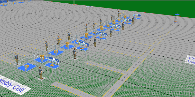
We modeled the digital twin of the electric transformer production line using actual data such as operation time per part and machine failure rates. Bottlenecks and inefficiencies were identified through multiple simulations. An algorithm using multiple fuzzy logic controllers were implemented to monitor performance and optimize machine combinations.
To do so, we proposed a fuzzy logic-based machine switching strategy for workers to increase the throughput of the production line by 12.5% in a 20 days of simulation run.
Video Demonstration:
Humanization in Task-oriented Conversational Agents
Human-Machine Conversational Interaction Project, Department of Electrical Engineering, University of Moratuwa
Tools: Python, NLP, LLM, Algorithms
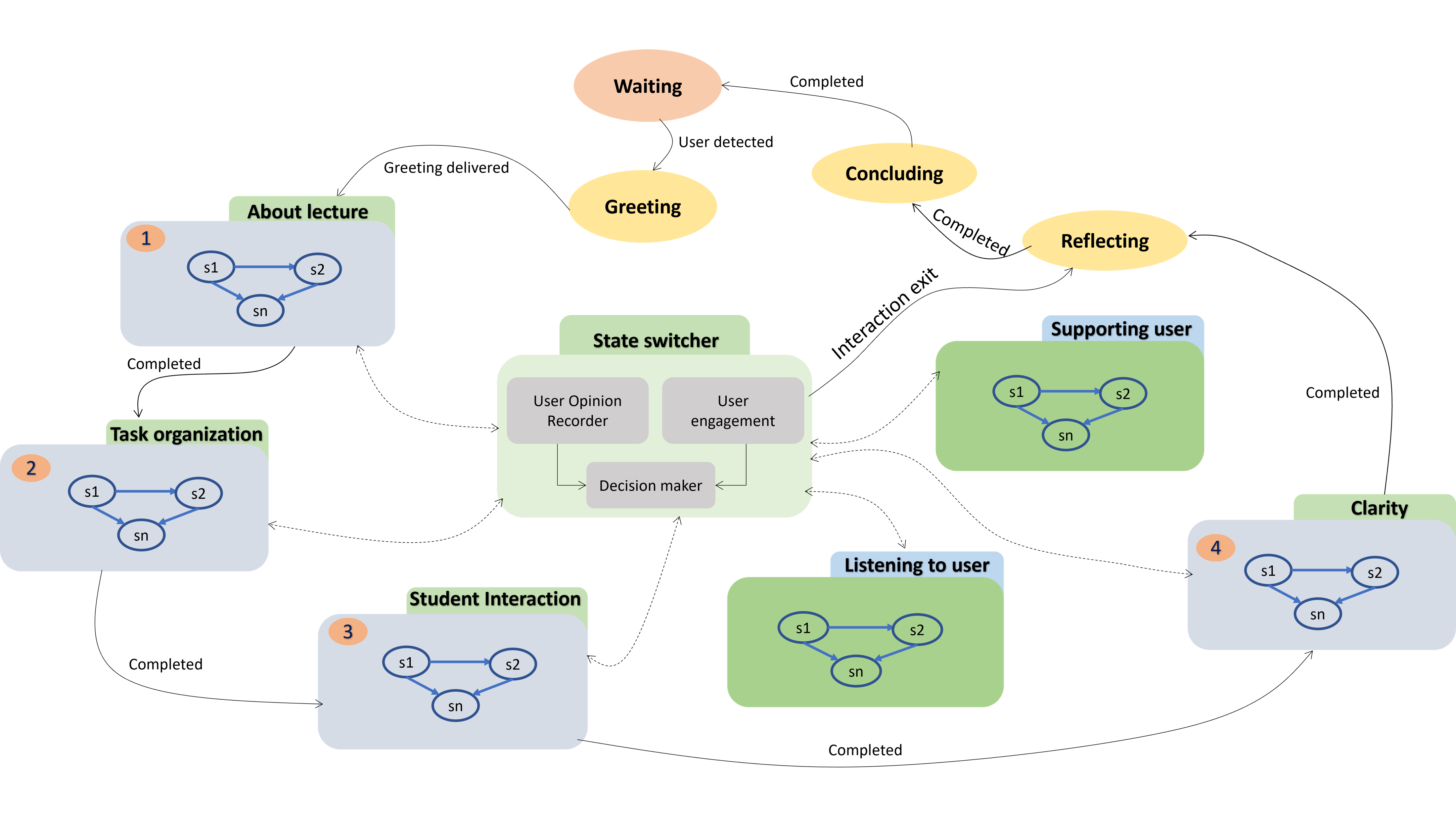
A short-term, extended task-oriented conversation system designed to gather user feedback about a lecture in a user-centered manner. The system leverages hierarchical state transitions to guide the conversation effectively.
How this system is different and serves your purpose?
A key advantage of this system is its adaptability to specific requirements. The pre-defined scripts utilized in the original implementation can be entirely replaced with your own custom scripts.
Key features include:
- State Management: The architecture currently supports a maximum of four "superstates."
- Survey Structuring: It is recommended to partition your survey questions into up to four main thematic blocks.
- Scalability: Each block can handle an unlimited number of individual questions.